Chapter 8: The Power of the Central Limit Theorem

Ever wonder why the normal distribution is ubiquitous? To answer this question, one must understand the power of the central limit theorem. The central limit theorem can be considered as the most profound but simple concept in the world of mathematics. This theorem applies to any type of distribution whether it is discrete or continuous. To explain the power of this theorem, it is best to look at the simulation shown below:

The simulation reveals the idea that the sample distribution of the sample means will form a shape of a normal distribution. This holds true regardless of the type of distribution examined. The number of sample sets that need to be collected in order to observe this trend is usually thirty which corresponds with the fact that the repeated sampling formula can only be applied when there are at least thirty samples.

Repeated sampling is also related to the central limit theorem because it states that the samples drawn from a normal population will form a normal distribution, when creating a distribution of sample means. This is the same as the power of the central limit theorem observed in the simulation above. However, the key difference between repeated sampling and the central limit theorem is that repeated sampling is limited to the fact that it only considers the normal distribution, or a distribution that is normalized, while the central limit theorem applies to all types of distribution. Hence, it is apparent that repeated sampling is part of the central limit theorem. The fact that, in the simulation above, the value of the mean is the same regardless of the n-value also supports the point that repeated sampling is related to the central limit theorem. Since, in repeated sampling, the population mean equals to any sample mean, regardless of the n-value (μ x bar= μ). Furthermore, the same pattern can be observed when finding the sum of the samples in each sample set.

In this way, the central limit theorem ties all types of distribution under the normal distribution.

Chapter 7: Poisson distribution: A Binomial Distribution without Success or Failure?

The binomial distribution consists of Bernoulli trials, hence success and failure is defined in order to calculate the probability. However, the Poisson distribution, known as a type of a binomial distribution, does not require the user to define success or failure. It is applied when determining the probability of a situation where we can expect something to happen for some amount of times during a specified interval. For example, if Ken usually receives five pieces of mail in his mailbox per day then he would be expecting to receive five mails every day. However, this does not mean that he will never receive more than or less than five mails, since the five mails that he has been expecting per day is just an expectation. In these kinds of situations, there will always be a certain spread, where Ken may only receive four mails, more than five or even none. Through applying the Poisson distribution, it is possible to find out the probability of a situation where we expect something to happen. However, the expected rate, also known as the average rate, and a certain time interval needs to be given in the question. The formula for the Poisson distribution is:

As shown, the Poisson distribution will generate the probability of how likely it is to get a certain value during a period of observation. In other words, it predicts the spread around a known average rate (expected rate) of occurrence. Even though the Poisson distribution helps solve certain problems, there are also limitations to this type of distribution. Firstly, the events must be repeated and independent so an outcome will not affect the result of the next outcome. Secondly, the fact that this is a discrete probability distribution also suggests that events need to be counted in whole numbers. Furthermore, as mentioned, the average rate, or the expected rate, and a specific time period needs to be known (the lambda value) in order to utilize the equation. Moreover, the formula can be applied when the question asks the probability of an event occurring, but, unlike binomial distributions, it cannot be applied to situations where it is asking for the probability of an event that will not occur. Last but not least, the Poisson distribution is a limited case of the binomial distribution. Although it does not require the user to define success, the p-value exists in problems that require the use of a Poisson distribution. When a Poisson distribution is applied, the probability of success (p-value) is a very small number. This is due to the fact that most of the time a person is expecting the expected outcome, so the probability of something that is not expected to happen occurring should be very low.

Chapter 3: Finding the Correlation Coefficient by Using the Slope of the Regression Line of z-scores

The correlation coefficient determines whether there is a linear relationship between two variables. However, the process of calculating the correlation coefficient is daunting especially in situations where the use of a calculator is prohibited. Yet, if one understands the splendid relationship between the slope of the regression line of z-scores and the correlation coefficient of the raw scores (which in this case are the x-values and the y-values before adjustments are made), the correlation coefficient can be determined without difficulty.

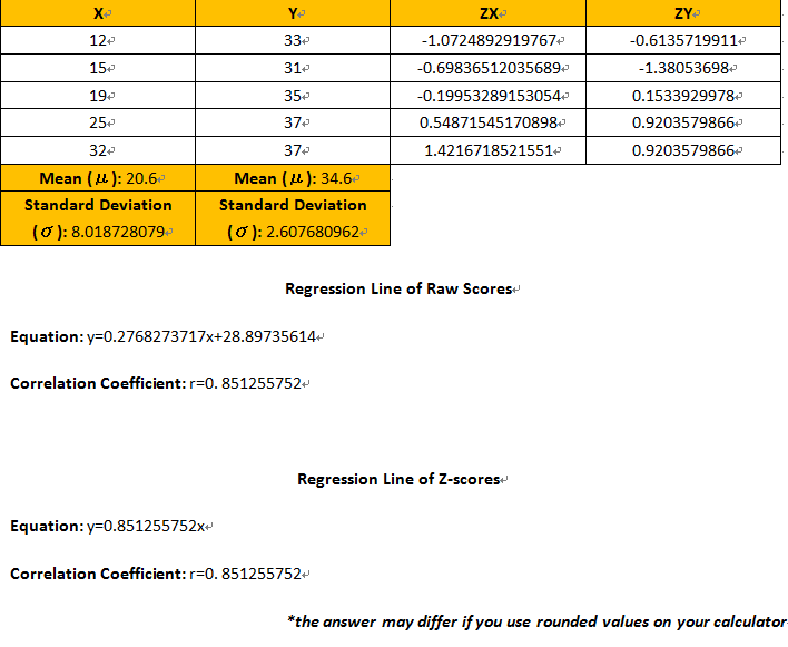
The calculation below will present the fact that the correlation coefficient of any linear regression is the slope of the linear regression of z-scores. The linear regression of z-scores is a linear regression found when converting all the independent and the dependent variables into z-scores. Therefore, when calculating the linear regression, the z-score values are used to formulate the regression. This also means that the larger the value of the correlation coefficient, the steeper the slope of the regression line of z-scores. The first two columns of the table shown below are the raw scores of the independent and dependent variables respectively. The third and the fourth column consist of independent and dependent variables that are transformed into z-score values.

As shown, the values of the correlation coefficient of the z-scores and the raw scores regression is equivalent, as well as the slope of the regression line of z-scores. This reveals the fact that the correlation coefficient is invariant when transforming independent and dependent variables to z-score values. Moreover, the slope of the regression line of z-scores is the correlation coefficient. Therefore, the equation of the linear regression of the z-scores is ZX= rZY or ZY= rZX. However, substituting ZX or ZY, from the table above, in these equations will not give the desired ZY or ZX values. This is due to the fact that the equation of the line is for the linear regression, so if the data points above are not located on the regression line, there is no way that substituting ZX or ZY values in the equation will lead to generating the desired amount.  Although we will not come across situations where we are not allowed to use our graphing calculators, understanding these kinds of relationships will certainly enhance our interest in the world of mathematics.

Chapter 2: Describing the Characteristics of a Data Set Using the Chebyshev’s Theorem

The measures of central tendency and spread are tools that can be applied to describe the characteristics of a set of data. Yet, for some data sets, these methods may not be enough to fully understand its nature. The Chebyshev’s theorem, invented by a Russian mathematician called Pafnuty Chebyshev, is a powerful concept that will add on to the list of characteristics that one can present while referring to a certain data set. When calculating the z-score for a particular datum, the value generated represents how many standard deviations the datum is away from the mean of the data group observed. However, the z-score does not indicate the number of datum that lies within a certain number of standard deviations away from the mean. This information is attainable through applying the Chebyshev’s theorem shown below.

As shown above, in order to apply the formula, the user must identify the k-value, which is the number of standard deviations away from the mean. This value, in a sense, is closely related to z-scores but in this case we are not looking at a specific datum, but a certain interval. The example below will clearly explain what is meant by this.

Notice that the example above does not state the number shots taken by Carol (the sample size, n-value). This is due to the fact that regardless of the number of shots taken, at least 75% of Carol’s shots will reach between 135m and 235m. During the process of calculation, only one end of the interval was chosen to calculate the k-value. It is unnecessary to pick both values at the end of each interval as long as the interval is equally apart. Since the Chebyshev’s theorem formula squares the k-value, thus meaning that negative values will become positive. Although the Chebyshev’s theorem does not generate the actual percentage of the data that lies within a given interval, it still is an indicator as to how far the data are spread out from the mean. Furthermore, this method applies to any set of data whether you are looking at discrete or continuous variables. Thus, when observing a set of data, this information is a useful characteristic that can be mentioned as long as the person identifies the appropriate interval. This can be done by developing an interval where most of the data tends to cluster around. For example, if I were to develop an interval for the set of data shown below, in this case, one possible solution would be to create the interval 20<x<30 because most of the data below tends to cluster around these numbers.

[21, 40, 50, 29, 25, 66, 77, 88, 30, 22, 26, 28, 29, 21]

Chapter 1: Finding the Inverse of a 3×3 Matrix and Solving a System of Linear Equations

Matrices are convenient tools that come in handy in various situations, from organizing large amounts of data to predicting long term trends. Even though matrices are utilized mostly in complex situations, there are also simpler ways to apply them. One unique and simple way to apply matrices is to solve linear equations with the aid of matrices. One might think that solving linear equations is simple, but from what I have seen many students tend to forget how to apply substitution or elimination to solve these types of equations.

As shown above, we are able to solve a system of linear equations using matrices. Although this method requires a lot of steps, it can also be used to solve linear equations with more than three variables. Hence, there should be quite a few situations where using matrices to solve linear equations may be an efficient approach compared to substitution or elimination. Furthermore, as you may have noticed, the number of rows and columns are the same as the number of variables. In the case shown above, there are three variables; therefore, there are three columns or rows (columns and rows for matrix A) in each matrix. Finding the inverse plays a huge part when solving linear equations using matrices. In class, we learned how to find the inverse of a 2×2 matrix, but the steps shown below need to be performed in order to find the inverse of a 3×3 matrix.

Although there are a couple of ways to find the inverse of a 3×3 matrix, this was the most understandable approach. The cofactor matrix, a type of matrix used to calculate the inverse and the determinant, has to be found in order to determine the adjugate matrix. This is because the adjugate matrix is the transpose of the cofactor matrix. Even though we have not explored these concepts in class, it is still possible to find the inverse of the 3×3 matrix as long as we understand the steps required to do so. Finding the inverse of a matrix with more than three rows and columns follows the same rule but is more complicated and requires additional steps; therefore, the use of calculator is strongly suggested for those types of situations.

Chapter 6: Regular Markov Chains with Zero Entries

The steady-state vector, a probability vector in the Markov chain, remains unchanged when it is multiplied by the transition matrix. The product should still equal the steady-state vector, even if the vector is multiplied to a transition matrix that has been raised to a power of a positive integer. In class, we have learned that if a transition matrix contains an entry of zero, it is not a regular Markov chain. According to the glossary section in the textbook, a regular Markov chain is “a Markov chain that always achieves a steady state”. Therefore, as long as we are able to find the steady-state vector of a transition matrix, a Markov chain can be considered regular, regardless of the entries in the transition matrix (excluding matrix with negative integers since we cannot have a percentage that is negative). The following question provides a situation where a transition matrix with zero entries will have a steady-state vector.

Question: Luigi, Daisy and Bowser are playing catch. Luigi always throws the ball to Daisy and Daisy always throws the ball to Bowser. Bowser throws the ball to Luigi 2/5 of the time and to Daisy 3/5 of the time. In the long run, what percentage of the time does each character receive the ball?

As shown above, it is possible to find the steady-state vector of a transition matrix that contains zero entries. Even though it is possible for some cases, it is also true that there are a lot of cases where the steady-state vector cannot be found. Another way to determine if a Markov chain is regular is to raise the transition matrix to a power of a positive integer and if the resulting matrix has all positive entries, this proves that it is a regular Markov chain. Figure 3 shows how this method can be used to determine whether a Markov chain is regular or not.

When attempting to find the steady-state vector for the transition matrix on the right (Figure 4), a row matrix was found.  If this row matrix was the steady-state vector, any initial probability vector multiplied by the transition matrix will eventually achieve a steady state. However, as you can see, the steady state cannot be not reached when the initial probability vector is given. Therefore, the transition matrix on the right does not have a steady-state vector, thus meaning that this transition matrix will not form a regular Markov chain. On the other hand, the transition matrix on the left has an entry of zero but has a steady-state vector. This is because the product of any initial probability vector and the transition matrix will always achieve a steady state. Therefore, from these examples, we can conclude that a regular Markov chain can have a transition matrix with an entry of zero.

Chapter 5: Venn diagrams Versus Euler Diagrams

Venn diagrams present the relationship between two or more things with clarity and simplicity. From experience, I feel that memorizing and understanding relationships become much easier with the aid of a Venn diagram. However, it is important to understand how Venn diagrams are drawn, especially when there are more than three sets involved. The diagrams below contain four circles but they are slightly different from each other in terms of the shape of the circles and the number of overlapping areas.

According to the Collins English Dictionary, a Venn diagram also known as a set diagram is “a diagram in which mathematical sets or terms of a categorial statement are represented by overlapping circles within a boundary representing the universal set, so that all possible combinations of the relevant properties are represented by the various distinct areas in the diagram.” As shown above, Figure 1 does not have any overlapping areas that cover only blue and red as well as only yellow and green. Therefore, according to the definition, Figure 1 is not a Venn diagram since it does not show all the possible combinations that should exist when comparing four sets. On the other hand, Figure 2 does show all the combinations, thus making it a Venn diagram.

“If Figure 1 is not a Venn diagram, then what is it?” This question was rolling around in my head, but was answered when I came across a diagram called the Euler diagram. The Euler diagram was invented by Leonhard Euler, a Swiss Mathematician and a physicist, to show the relationship between two or more things. From this explanation, Venn diagrams and Euler diagrams can be interpreted as the same diagram. However, the key difference between these two diagrams is that an Euler diagram only shows the relationships that exist, while a Venn diagram shows all the possible relationships, meaning that it even depicts the relationships that are unfeasible. The subset and disjoint in Figure 3 and 4 will help assist in understanding the difference between the two.

The unfeasible area in the Venn diagram represents the null set which is a set that is empty

As shown above, in order to present a subset and a disjoint in a Venn diagram, the overlapping areas without any elements also need to be presented. This is because Venn diagrams present all combinations even if they are unfeasible. If not, then it is an Euler diagram, because Euler diagrams only show the relationships that exist.

Chapter 4: Polygonal Numbers and the Pascal’s Triangle

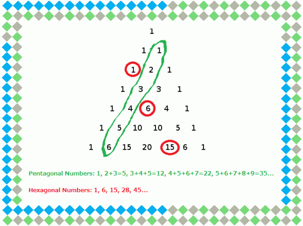
The Pascal’s triangle is filled with mathematical patterns such as the triangular numbers and the square numbers. While studying these patterns, I noticed that the pentagonal numbers and the hexagonal numbers also exist within the triangle. The pentagonal numbers are numbers that can be shown as a pentagonal pattern of dots, whereas the hexagonal numbers are numbers that form a hexagonal pattern. For both patterns, the number of dots required to create the next smallest shape determines the next number in the pattern (See Chart 1 below). The sums of adjacent counting numbers, found in the second diagonal of the Pascal’s triangle, are the pentagonal numbers. However, the number of counting numbers added at a time depends on each pentagonal number (EX. 1, 2+3=5, 3+4+5=12, 4+5+6+7=22, 5+6+7+8+9=35). Hexagonal numbers can be spotted easily, since every odd triangular number (the 1^st, 3^rd, 5^th… triangular number) is a hexagonal number.

In class we learned that the n^th triangular number is the sum of the first n positive integers. Thus, it also means that the numbers added to get the next triangular number is always increasing by one. For square numbers, the number that needs to be added in order to get the next number is two, three for pentagonal numbers and four for hexagonal numbers. Therefore, the numbers added in order for the next smallest shape to form increases by one for each different pattern. This is because in order for the next smallest shape to form, the sides of a given shape will have to be longer than the previous shape by exactly one dot.  The number of sides also affects the pattern because a square will always have one additional side than the triangle, a pentagon will always have one additional side than the square and a hexagon will always have one additional side than the pentagon.

As you can see, the numbers added in order for the next smallest shape to form increases by one for each different pattern (there is always one additional dot added in order to create the next smallest triangle, but two dots are added for squares, three for pentagons, and four for hexagons).
This is because the sides of a given shape will have to be longer than the previous shape by exactly one dot (the 2nd shape always has two dots for each side, the 3rd shape has three dots, the 4th shape has four dots, and the 5th shape has five dots).

Odd and Even Pattern
The sequence is odd, odd, even, even, odd, odd, even, even,… for triangular numbers and pentagonal numbers.
The sequence is odd, even, odd, even, odd, even… for square numbers and hexagonal numbers.